2.1 Using R’s built-in datasets and “viewing” datasets

Take a look at the Environment tab in the top right pane. Any datasets that you import into R or any loaded datasets (that come with R) will appear in this tab. In this course, we will either import a dataset that is stored in a .csv file or using a dataset that already comes with R (by way of an R package. Here, we illustrate using a dataset that already comes with R. The dataset is the resulting measurements from an experiment on the effect of diet on early growth of chicks.

R refers to this dataset as ChickWeight. We can look at this data by first telling *R that we want to use it by using following command:

data( ChickWeight )  # this tells R that we want to use the 'ChickWeight` data
# It should now appear in R's memory (see Environment tab)
# Note: This command may open a spreadsheet of the data in
# a new tab.  Simply close the tab and return to your R script
# file.

We can now look at the data within the console by typing its name in the R script, highlighting it, and selecting “Run”

ChickWeight 

It’s going to print a lot of data (578 rows of it). To view the data in a spreadsheet, click on the name ChickWeight in the Environment tab (upper right pane). This will open a spreadsheet of the data in a new tab in the source pane.

What you should see in the spreadsheet are four columns of numbers, each row representing a chick measured: the first entry in each row is simply the row number (an index we can use to access the data from individual chicks if we want), the second is the weight (body weight of the chick), the third is Time (number of days since birth) , the fourth Chick (an identifier for the chick), and the fifth is Diet (experimental diet the chick received: Diet 1 , 2, 3, or 4). You can use the scroll bar on the right side of the console window to examine the complete data set.

Alternatively, to open the data spreadsheet, one can instead run:

View( ChickWeight ) 

Note that the row numbers in the first column are not part of ChickWeight’s data. R adds them as part of its printout to help you make visual comparisons. You can think of them as the index that you see on the left side of an Excel spreadsheet. In fact, the comparison to a spreadsheet will generally be helpful. R has stored ChickWeight dataset in a kind of spreadsheet or table called a dataframe. Rather than looking at the spreadsheet of the data, we can instead explore the dataframe in various way to extract useful characteristics. For example, one can see how many variables (chick characteristics of interest) were measured/recorded and the number of observations on these variables by running:

require( mosaic ) # tell R we want to use the mosaic package

glimpse( ChickWeight )

The R function/command called glimpse( ) is part of the mosaic package. This is why one has to first run require( mosaic )

In general, datasets that come with R or an R package, such as ChickWeight have what is called a help file that will provide details regarding the data set. Help files are disscuseed later in this chapter.

2.2 .csv files

It is assumed you have used an excel spreadsheet. If not, please view the tutorial Excel Tutorial for Beginners .

Data sets used in this class will either be built-in datasets (that is, they come with R or from an R package) or they will be .csv files. A .csv may be viewed with Microsoft Excel. We will import .csv files into RStudio. If you have data that you want to import into RStudio, you will first store your data in a .csv file using Excel. The format in which you store it should be a data matrix or in tidy form. There are three characteristics that make a dataset a data matrix or tidy:

• Each variable must have its own column.
• Each observation must have its own row.
• Each value must have its own cell.

To setup your spreadsheet, do the following steps:

• Step 1 – Input and organize your data in Excel.
  • Organize your data in an Excel worksheet, such that the first row (Row 1) contains the column names and each subsequent row contains all the necessary information for each data point. For example:

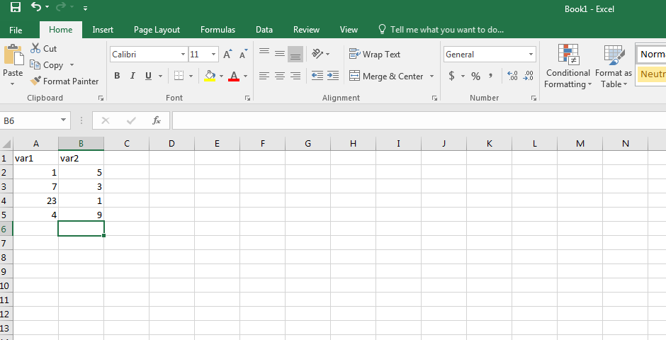
Figure 2.1

• Step 2 – Save your worksheet as a comma separated values (.csv) file type. Select the following Excel tabs File>Save As, then select where you want to save your .csv file. A window will appear in which one can specify their desired filename as well as their desired file type. Enter a file name and click on “Save as type” and scroll down to select CSV (Comma delimited) (see figure below).

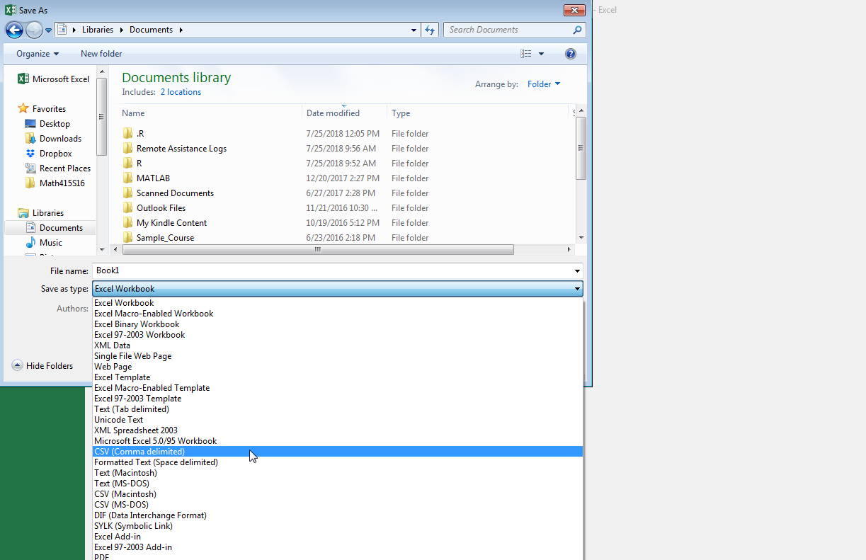
Figure 2.2

When you click to save the worksheet as a comma separated file (.csv), Excel may present you with a one or two warnings. One may warn you that the .csv format cannot accommodate multiple worksheets. That’s fine; just click “Yes” to save the active worksheet. The second warning tells you that “Some features in your workbook might be lost if you save it as a CSV (Comma delimited).” Again, that’s fine, just click “Yes”. When you’re done, you will see that a new file has been created in the directory where you saved your file. If you were to open this file in excel you would see your spreadsheet with the data you entered. On the surface, it looks no different than an excel spreadsheet file (.xls or .xlsx)

Important: Any .csv file that you plan to import into R must have the first row (Row 1) contain the column names and each subsequent row contains all the necessary information for each data point.

2.3 Importing a .csv file

We will use the R function read.csv() to import data into RStudio. We illustrate the method using the “MLB salaries (2010)” data set and this data is stored in a .csv file. This .csv file is located at the following url: http://www.csub.edu/~emontoya2/datasets/mlb2010.csv

To import the data into RStudio, we use read.csv() and it is a simple function to use. It just requires the location of the file. If the data location is a url, then use the url. If it is data that you’ve created or recorded and it is saved on your computer, then we use file.choose(). We will cover both methods here.

mlbDataImport = read.csv( "http://www.csub.edu/~emontoya2/datasets/mlb2010.csv" )

2.3.2 Importing data from your computer

Download the .csv file below onto your computer. Make sure to note where your file is saved. Depending on your browser settings, after clicking on the link below, the file will either open in your browser and it will be downloaded.

http://www.csub.edu/~emontoya2/datasets/sampledata.csv

After saving this .csv file, run the following

### by putting in "file.choose()", this tells R that you want 
### to browse for and select the csv file
ImportFromDrive = read.csv( file.choose() )

This automatically opens a window that allows you to browse for your .csv file. Select your file and click on Open. You should see the following in the console

Figure 2.3

The data set ImportFromDrive should appear in the Environment tab in the upper right panel where it displays the number of observations and variables.

Note: Data that you import will not have help files. Only datasets that come with R (or from R packages) have help files.

2.4 Summarizing data

There are many ways to summarize data in R. We will be using functions from the mosaic package. From hereafter, always load the mosaic package. That is, always have the following in your R script before writing any commands to conduct any analysis:

require( mosaic )

When wanting to summarize a single variable, the formula to create graphical and numerical summaries follows the general form goal( ~ x , data) where x is the variable you want to graph or compute a statistic of. Depending on the summary, we may have to specify some additional things. If the variable x is a variable in the dataframe/dataset, then data would be set equal to the name of the data frame. The names used for x and the name of the dataframe must be the names that R has given the data set and variable. goal would be replaced with the name of the function.

Recall that we imported the MLB dataset and we stored it in a dataframe called mlbDataImport. Let’s take a glimpse at the data

glimpse( mlbDataImport )  # this function is from the mosaic package
#> Rows: 828
#> Columns: 4
#> $ player   <chr> "Brandon Webb", "Danny Haren", "Chris Snyder", "Edwin Jackson~
#> $ team     <chr> "Arizona Diamondbacks", "Arizona Diamondbacks", "Arizona Diam~
#> $ position <chr> "Pitcher", "Pitcher", "Catcher", "Pitcher", "First Baseman", ~
#> $ salary   <dbl> 8500.000, 8250.000, 5250.000, 4600.000, 4500.000, 4185.000, 3~

Let’s start with a simple graphical summary. R has three plotting systems: base, lattice, and ggplot2. We will be using the lattice system, which comes from the lattice package. This package is automatically installed when you installed the mosaic package, and this package is automatically loaded when you loaded the mosaic package (require( mosaic )).

To start, a histogram of salary will created. salary represents the salary (in $1000s) of a given baseball player in 2010. Again, the basic formula is goal( ~ x , data) where goal would be replaced with the name of the function to create the desired graph. R refers to histograms as histogram():

histogram( ~ salary  , data=  mlbDataImport )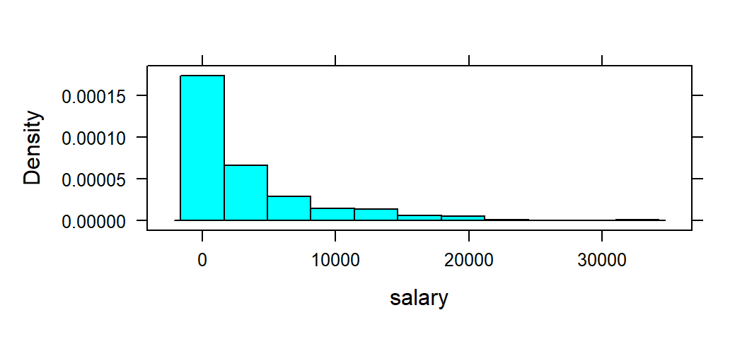 

Let’s compute the mean salary of these baseball players. Again, salary represents the salary of a given baseball player in 2010. As with the graph, the basic formula is goal( ~ x , data) where goal would be replaced with the name of the function to compute the desired sample statistic. To compute the mean, R calls its function mean:

mean( ~ salary  , data=  mlbDataImport )
#> [1] 3281.828

Suppose you wanted to compute the average salary for each position. To so, we can tell RStudio to compute the mean by levels/groups of a grouping variable. A grouping variable groups data into categories or groups. Grouping variables are categorical variables. When summaries are desired based on the levels or groups of the grouping variables, they are called side-by-side or comparative summaries.

For any side-by-side or comparative data summary, the general formula changes a bit. The formula is goal( ~ x | gfactor , data), where gfactor represent the grouping variable. In our example, the grouping variable is position:

mean( ~ salary | position , data=  mlbDataImport )
#>           Catcher Designated Hitter     First Baseman         Infielder 
#>          1937.220          5235.714          5826.521           770.575 
#>        Outfielder           Pitcher    Second Baseman         Shortstop 
#>          3753.926          2999.197          3022.723          2844.146 
#>     Third Baseman 
#>          4641.286

One may also create a side-by-side or comparative graphical summary. To create a boxplot of salary for each position, run the following:

bwplot( ~ salary | position , data=  mlbDataImport )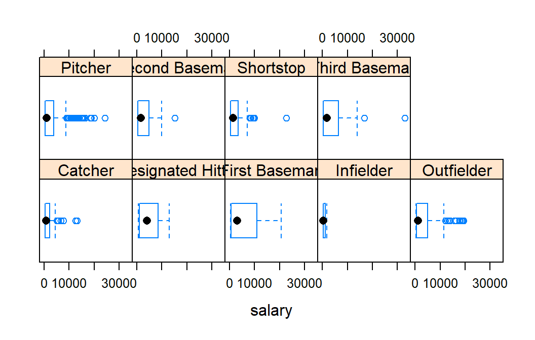

2.5 Export an R plot or R output

2.5.1 Exporting graphs

One may need to create a graph or one may have to submit RStudio output for certain assignment or exam problems. To export a plot, go to the Plots tab in the bottom right panel, click on Export>….

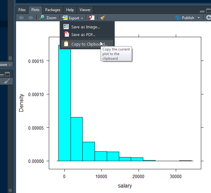
Figure 2.4

You have three export format options:

• “Save as Image…”
• “Save as PDF…”
• “Copy to Clipboard…”

Select your preferred option. A small window should then appear of the plot. In the pop up window you may adjust the size of the plot and provide a name for the new file (see below for an example when one selects “Copy to Clipboard…”).

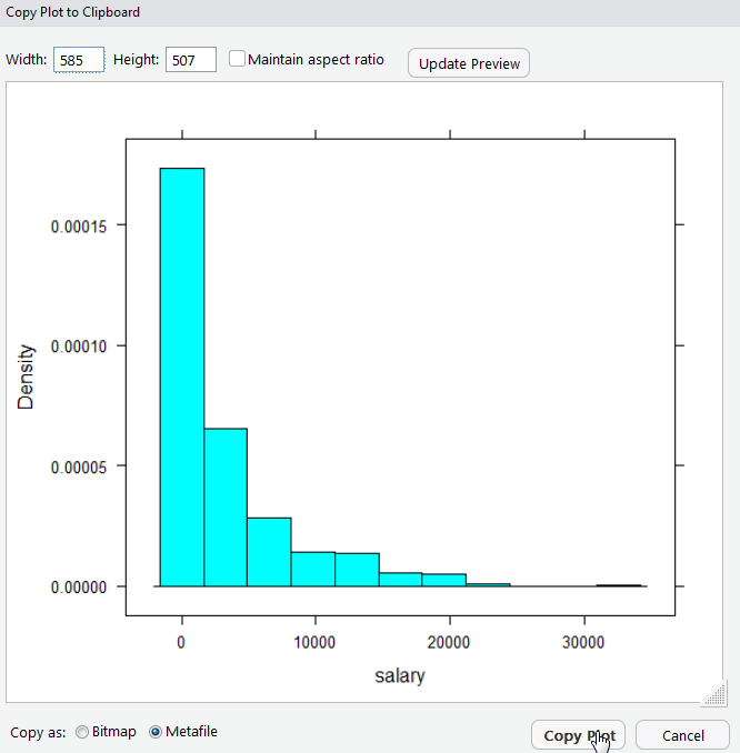
Figure 2.5

2.6 Extracting variables from dataframes

To extract a given variable from a dataframe, we place a $ at the end of the dataframe name, followed by the variable name. To illustrate, we use R’s built-in dataset called trees, which contains the diameter, height and volume for 31 cherry trees:

glimpse( trees )
#> Rows: 31
#> Columns: 3
#> $ Girth  <dbl> 8.3, 8.6, 8.8, 10.5, 10.7, 10.8, 11.0, 11.0, 11.1, 11.2, 11.3, ~
#> $ Height <dbl> 70, 65, 63, 72, 81, 83, 66, 75, 80, 75, 79, 76, 76, 69, 75, 74,~
#> $ Volume <dbl> 10.3, 10.3, 10.2, 16.4, 18.8, 19.7, 15.6, 18.2, 22.6, 19.9, 24.~

To extract the variable Volume, do the following:

trees$Volume 
#>  [1] 10.3 10.3 10.2 16.4 18.8 19.7 15.6 18.2 22.6 19.9 24.2 21.0 21.4 21.3 19.1
#> [16] 22.2 33.8 27.4 25.7 24.9 34.5 31.7 36.3 38.3 42.6 55.4 55.7 58.3 51.5 51.0
#> [31] 77.0

### Lets store the volume measurements
### into an R objects called 'treeVol'.
### We can then call 'treeVol' whenever
### we need to use these measurements.
treeVol <- trees$Volume # assign vol. meas. to 'treeVol'

2.7 Understanding common R errors

Everyone gets errors in R. It’s part of the process of learning any new software. Here are some of the most common error you may encounter and what they mean

> whatIsThis( 4 ) # no such function/command exist
Error in whatIsThis(4) : could not find function "whatIsThis"

mean( ~ salary  , data=  mlbDataImport )
#> [1] 3281.828

> Mean( ~ salary  , data=  mlbDataImport )
Error in Mean(~salary, data = mlbDataImport) : 
  could not find function "Mean"

> MlbDataImport
Error: object 'MlbDataImport' not found

> histogram( ~ salary  , data=  mlbDataImport ) ) ) 
Error: unexpected ')' in "histogram( ~ salary  , data=  mlbDataImport ) )

> histogram( ~ salary  , data=  mlbDataImport 
+ 
+ 
+ 
+ 
### Hit the 'Esc' key a few times to have
### R stop prompting.  

2.8 Help files

All built in functions, as well as data sets, in R have help files. To access the help files for a function or data set one uses the function help( ). In general, the help file will contain the following sections:

• Description: Gives brief description of the function.
• Usage: Displays a functions arguments, along with the default values of certain arguments.
• Arguments: Gives details of each of the functions arguments.
• Value: Describes what is returned by the function.
• See Also: Lists links to help files of similar functions.
• Example: Gives example code that uses the function(s).

For example, the following commands bring up the help file on the log( ) function,

> help(log)
Help for 'log' is shown in the browser
> ?log  # This is equivalent to help(log)
Help for 'log' is shown in the browser
>

Either of these commands should open the following (abbreviated) help file

log {base}                                 R Documentation

Logarithms and Exponentials Description

log computes natural logarithms, log10 computes common (i.e., base 10)
logarithms, and log2 computes binary (i.e., base 2) logarithms.
The general form logb(x, base) computes logarithms with base base.

Usage:
  
log(x, base = exp(1))
logb(x, base = exp(1))
log10(x)
log2(x)

Arguments:
  
  x       a numeric or complex vector.
base    positive number. The base with respect to which logarithms
are computed. Defaults to e=exp(1).

Value:
  
  A vector of the same length as x containing the transformed
values. log(0) gives -Inf (when available).

...

Examples:
  
  log(exp(3))
log10(1e7)# = 7

The function log() has two arguments. The first is a numeric vector and the second corresponds to the base. By default the function log() will evaluate with an exponential base unless you specify otherwise as illustrated below.

> log(10)
[1] 2.302585
> log(10, base = exp(1))
[1] 2.302585
> log(10, base = 2)
[1] 3.321928
>

If you seek an example of using a given function, it is a good idea to look at the examples given at the end of the help file. Now suppose you had no idea that a logarithm function existed, but you would like to know if such a function might exist in R. To explore this question you can issue help.search( "logarithm" ) which will search the help files for documentation matching the character string logarithm. You may also run RSiteSearch( "logarithm" ) which will search for the character string “logarithm” in the R-help mailing list archives. Lastly, you can do a web search for your error as it is almost certain someone has had the same or similar error.